14 R Markdown

By the end of this lesson, you will be able to:
- Understand the basics of R Markdown
- Create documents that combine code, output, and narrative text
- Format text using Markdown syntax
- Generate reports in multiple formats (HTML, PDF, Word)
- Use R Markdown for reproducible data analysis
1 What is R Markdown?
R Markdown is a file format that allows you to combine R code, its output, and narrative text in a single document. It’s a powerful tool for creating reproducible reports, presentations, dashboards, and even websites.
R Markdown documents are plain text files that contain three important elements: 1. YAML header - Document metadata and formatting options 2. Markdown text - For narrative content 3. Code chunks - R code that can be executed
2 Getting Started with R Markdown
To create an R Markdown document in RStudio:
- Click File → New File → R Markdown
- Choose a document type (HTML, PDF, or Word)
- Give your document a title and author name
- Click OK
This will generate a template R Markdown file that you can modify.
3 YAML Header
The YAML header appears at the top of the document between triple dashes (---):
---
title: "My Analysis Report"
author: "Your Name"
date: "2023-06-15"
output: html_document
---
You can customize various aspects of your document by adding options to the YAML header:
---
title: "My Analysis Report"
author: "Your Name"
date: "2025-07-09"
output:
  html_document:
    toc: true
    toc_float: true
    theme: flatly
    highlight: tango
    code_folding: show
---
4 Markdown Text
Markdown is a lightweight markup language that allows you to format text using simple syntax:
4.1 Basic Formatting
# Heading 1
## Heading 2
### Heading 3
**Bold text**
*Italic text*
~~Strikethrough~~
[Link text](https://example.com)
4.2 Lists
Unordered list:
- Item 1
- Item 2
  - Subitem 2.1
  - Subitem 2.2

Ordered list:
1. First item
2. Second item
   a. Subitem a
   b. Subitem b
4.3 Tables
| Column 1 | Column 2 | Column 3 |
|----------|----------|----------|
| Row 1    | Data     | Data     |
| Row 2    | Data     | Data     |
5 Code Chunks
Code chunks in R Markdown allow you to execute R code and display its results:
::: {.cell}

```{.r .cell-code}
# Your R code here
```
:::
For example:
::: {.cell}

```{.r .cell-code}
# Load data
data(mtcars)

# Calculate summary statistics
summary(mtcars)
```

::: {.cell-output .cell-output-stdout}

```
      mpg             cyl             disp             hp
 Min.   :10.40   Min.   :4.000   Min.   : 71.1   Min.   : 52.0
 1st Qu.:15.43   1st Qu.:4.000   1st Qu.:120.8   1st Qu.: 96.5
 Median :19.20   Median :6.000   Median :196.3   Median :123.0
 Mean   :20.09   Mean   :6.188   Mean   :230.7   Mean   :146.7
 3rd Qu.:22.80   3rd Qu.:8.000   3rd Qu.:326.0   3rd Qu.:180.0
 Max.   :33.90   Max.   :8.000   Max.   :472.0   Max.   :335.0
      drat             wt             qsec             vs
 Min.   :2.760   Min.   :1.513   Min.   :14.50   Min.   :0.0000
 1st Qu.:3.080   1st Qu.:2.581   1st Qu.:16.89   1st Qu.:0.0000
 Median :3.695   Median :3.325   Median :17.71   Median :0.0000
 Mean   :3.597   Mean   :3.217   Mean   :17.85   Mean   :0.4375
 3rd Qu.:3.920   3rd Qu.:3.610   3rd Qu.:18.90   3rd Qu.:1.0000
 Max.   :4.930   Max.   :5.424   Max.   :22.90   Max.   :1.0000
       am              gear            carb
 Min.   :0.0000   Min.   :3.000   Min.   :1.000
 1st Qu.:0.0000   1st Qu.:3.000   1st Qu.:2.000
 Median :0.0000   Median :4.000   Median :2.000
 Mean   :0.4062   Mean   :3.688   Mean   :2.812
 3rd Qu.:1.0000   3rd Qu.:4.000   3rd Qu.:4.000
 Max.   :1.0000   Max.   :5.000   Max.   :8.000
```


:::
:::
5.1 Chunk Options
You can control how code chunks behave using options:
| Option | Description |
|---|---|
eval=TRUE/FALSE |
Whether to evaluate the code |
echo=TRUE/FALSE |
Whether to show the code |
include=TRUE/FALSE |
Whether to include the chunk in output |
message=TRUE/FALSE |
Whether to display messages |
warning=TRUE/FALSE |
Whether to display warnings |
fig.width=7 |
Figure width in inches |
fig.height=5 |
Figure height in inches |
Example:
#```{r plot, fig.width=8, fig.height=4, echo=FALSE}
# Create a plot without showing the code
plot(mtcars$wt, mtcars$mpg,
     main="Car Weight vs. Mileage",
     xlab="Weight (1000 lbs)",
     ylab="Miles Per Gallon",
     pch=19, col="blue")
#```
6 Inline Code
You can also include R code directly within text using backticks and r:
# The average miles per gallon is <backtick>r mean(mtcars$mpg)<backtick>.
The average miles per gallon is 20.090625.
This will calculate the mean and insert the result directly into your text.
7 Generating Reports
To generate your report:
- Click the Knit button in RStudio
- Choose your desired output format
- View the generated document
R Markdown will: - Run all the code chunks - Generate all outputs (tables, plots, etc.) - Format the text according to Markdown syntax - Combine everything into a single document
8 Example: Data Analysis Report
Here’s a simple example of an R Markdown document for data analysis:
---
title: "Car Performance Analysis"
author: "Data Scientist"
date: "2025-07-09"
output: html_document
---
### Introduction
This report analyzes the relationship between car characteristics and fuel efficiency.
### Data Overview
::: {.cell}
```{.r .cell-code}
# Load the mtcars dataset
data(mtcars)
# Display the first few rows
head(mtcars)
```
::: {.cell-output .cell-output-stdout}
```
mpg cyl disp hp drat wt qsec vs am gear carb
Mazda RX4 21.0 6 160 110 3.90 2.620 16.46 0 1 4 4
Mazda RX4 Wag 21.0 6 160 110 3.90 2.875 17.02 0 1 4 4
Datsun 710 22.8 4 108 93 3.85 2.320 18.61 1 1 4 1
Hornet 4 Drive 21.4 6 258 110 3.08 3.215 19.44 1 0 3 1
Hornet Sportabout 18.7 8 360 175 3.15 3.440 17.02 0 0 3 2
Valiant 18.1 6 225 105 2.76 3.460 20.22 1 0 3 1
```
:::
```{.r .cell-code}
# Summary statistics
summary(mtcars[, c("mpg", "wt", "hp")])
```
::: {.cell-output .cell-output-stdout}
```
mpg wt hp
Min. :10.40 Min. :1.513 Min. : 52.0
1st Qu.:15.43 1st Qu.:2.581 1st Qu.: 96.5
Median :19.20 Median :3.325 Median :123.0
Mean :20.09 Mean :3.217 Mean :146.7
3rd Qu.:22.80 3rd Qu.:3.610 3rd Qu.:180.0
Max. :33.90 Max. :5.424 Max. :335.0
```
:::
:::
### Visualization
::: {.cell}
```{.r .cell-code}
# Create a scatterplot
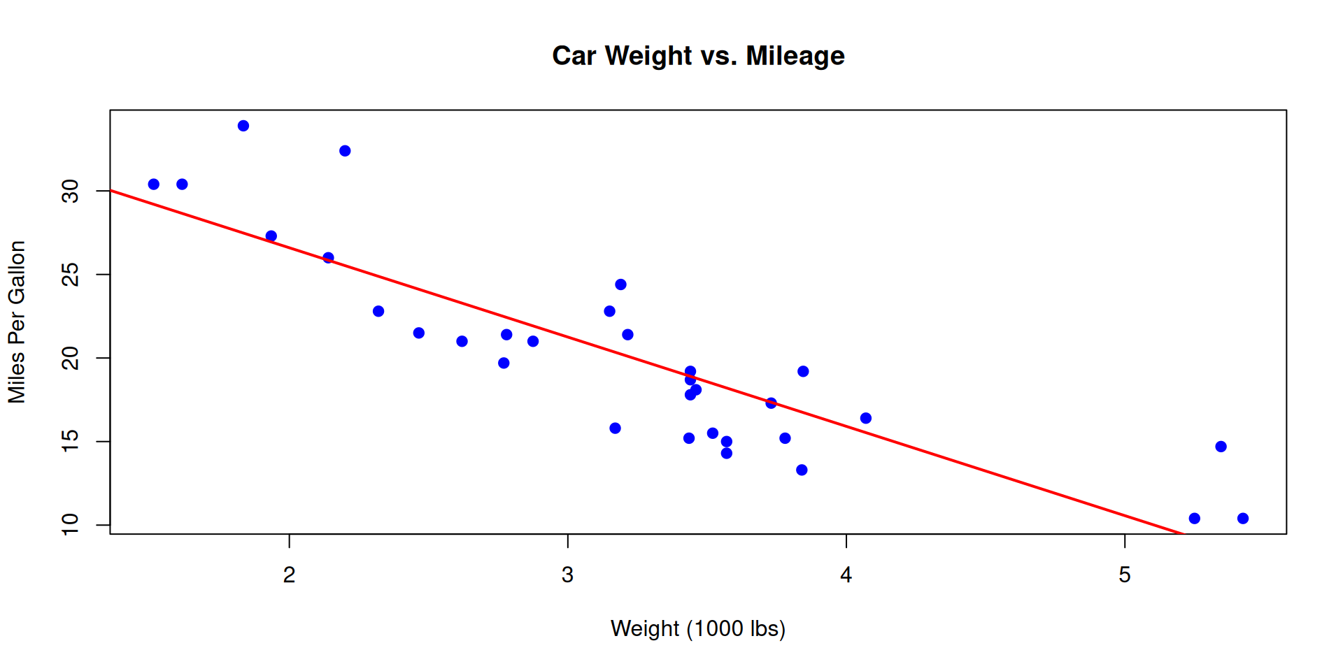
plot(mtcars$wt, mtcars$mpg,
main="Car Weight vs. Mileage",
xlab="Weight (1000 lbs)",
ylab="Miles Per Gallon",
pch=19, col="blue")
# Add a regression line
abline(lm(mpg ~ wt, data = mtcars), col = "red", lwd = 2)
```
::: {.cell-output-display}
{width=960}
:::
:::
### Statistical Analysis
::: {.cell}
```{.r .cell-code}
# Fit a linear model
model <- lm(mpg ~ wt + hp, data = mtcars)
# Display model summary
summary(model)
```
::: {.cell-output .cell-output-stdout}
```
Call:
lm(formula = mpg ~ wt + hp, data = mtcars)
Residuals:
Min 1Q Median 3Q Max
-3.941 -1.600 -0.182 1.050 5.854
Coefficients:
Estimate Std. Error t value Pr(>|t|)
(Intercept) 37.22727 1.59879 23.285 < 2e-16 ***
wt -3.87783 0.63273 -6.129 1.12e-06 ***
hp -0.03177 0.00903 -3.519 0.00145 **
---
Signif. codes: 0 '***' 0.001 '**' 0.01 '*' 0.05 '.' 0.1 ' ' 1
Residual standard error: 2.593 on 29 degrees of freedom
Multiple R-squared: 0.8268, Adjusted R-squared: 0.8148
F-statistic: 69.21 on 2 and 29 DF, p-value: 9.109e-12
```
:::
:::
### Conclusion
Based on our analysis, there is a significant negative relationship between car weight and fuel efficiency. For every 1,000 lb increase in weight, the miles per gallon decreases by approximately 3.88 units.9 Practice Exercises
9.1 Basic R Markdown
Create a new R Markdown document that includes: - A title and your name - A brief introduction - A code chunk that loads and summarizes a dataset of your choice - A visualization of the data - A brief conclusion
Here’s an example of a basic R Markdown document:
---
title: "Analysis of Iris Dataset"
author: "Your Name"
date: "2025-07-09"
output: html_document
---
## Introduction
This document provides a brief analysis of the iris dataset, which contains measurements of sepal length, sepal width, petal length, and petal width for three species of iris flowers: setosa, versicolor, and virginica.
## Data Summary
::: {.cell}
```{.r .cell-code}
# Load the iris dataset
data(iris)
# Display the structure of the dataset
str(iris)
```
::: {.cell-output .cell-output-stdout}
```
'data.frame': 150 obs. of 5 variables:
$ Sepal.Length: num 5.1 4.9 4.7 4.6 5 5.4 4.6 5 4.4 4.9 ...
$ Sepal.Width : num 3.5 3 3.2 3.1 3.6 3.9 3.4 3.4 2.9 3.1 ...
$ Petal.Length: num 1.4 1.4 1.3 1.5 1.4 1.7 1.4 1.5 1.4 1.5 ...
$ Petal.Width : num 0.2 0.2 0.2 0.2 0.2 0.4 0.3 0.2 0.2 0.1 ...
$ Species : Factor w/ 3 levels "setosa","versicolor",..: 1 1 1 1 1 1 1 1 1 1 ...
```
:::
```{.r .cell-code}
# Summary statistics
summary(iris)
```
::: {.cell-output .cell-output-stdout}
```
Sepal.Length Sepal.Width Petal.Length Petal.Width
Min. :4.300 Min. :2.000 Min. :1.000 Min. :0.100
1st Qu.:5.100 1st Qu.:2.800 1st Qu.:1.600 1st Qu.:0.300
Median :5.800 Median :3.000 Median :4.350 Median :1.300
Mean :5.843 Mean :3.057 Mean :3.758 Mean :1.199
3rd Qu.:6.400 3rd Qu.:3.300 3rd Qu.:5.100 3rd Qu.:1.800
Max. :7.900 Max. :4.400 Max. :6.900 Max. :2.500
Species
setosa :50
versicolor:50
virginica :50
```
:::
:::
## Data Visualization
::: {.cell}
```{.r .cell-code}
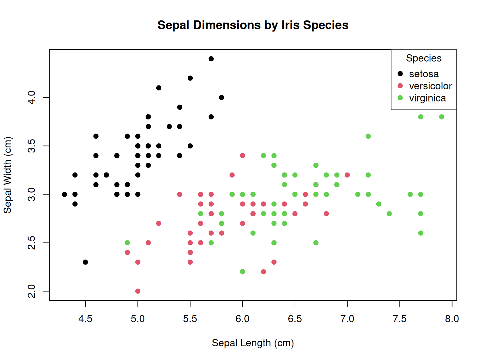
# Create a scatterplot of sepal dimensions by species
plot(iris$Sepal.Length, iris$Sepal.Width,
main = "Sepal Dimensions by Iris Species",
xlab = "Sepal Length (cm)",
ylab = "Sepal Width (cm)",
pch = 19,
col = as.numeric(iris$Species))
# Add a legend
legend("topright",
legend = levels(iris$Species),
col = 1:3,
pch = 19,
title = "Species")
```
::: {.cell-output-display}
{width=768}
:::
:::
## Conclusion
The visualization reveals clear clustering of iris species based on sepal dimensions. Setosa irises (shown in black) have shorter sepals that are wider, while versicolor (red) and virginica (green) have longer, narrower sepals. This simple analysis demonstrates how morphological measurements can be used to distinguish between iris species.This R Markdown document includes: 1. A YAML header with title, author, and date 2. A brief introduction to the dataset 3. A code chunk that loads and summarizes the iris dataset 4. A visualization showing the relationship between sepal dimensions by species 5. A brief conclusion interpreting the visualization
9.2 Output Formats
Experiment with different output formats (HTML, PDF, Word) and observe the differences.
To experiment with different output formats, you would modify the YAML header of your R Markdown document as follows:
For HTML output:
---
title: "My Analysis"
author: "Your Name"
date: "2025-07-09"
output: html_document
---
For PDF output:
---
title: "My Analysis"
author: "Your Name"
date: "2025-07-09"
output: pdf_document
---
For Word output:
---
title: "My Analysis"
author: "Your Name"
date: "2025-07-09"
output: word_document
---
For multiple output formats:
---
title: "My Analysis"
author: "Your Name"
date: "2025-07-09"
output:
  html_document:
    toc: true
    toc_float: true
  pdf_document:
    toc: true
  word_document:
    toc: true
---
Key differences between formats:
-
HTML:
- Most interactive and customizable
- Supports interactive elements (e.g., plotly plots, shiny apps)
- Easy to share online
- Supports custom CSS styling
- Includes features like floating table of contents and code folding
-
PDF:
- More formal appearance, suitable for printing
- Requires LaTeX installation (TinyTeX recommended)
- Better for precise layout control
- Good for academic papers and reports
- May have issues with very large tables or complex plots
-
Word:
- Familiar format for non-technical collaborators
- Easy for others to edit and add comments
- Good for documents that need further editing
- Limited in terms of formatting control compared to HTML/PDF
- May have inconsistent rendering of complex elements
To fully experience these differences, you would need to knit the same document to each format and compare the results.
9.3 Advanced Features
Create an R Markdown document with a table of contents, code folding, and a custom theme.
Here’s an example of an R Markdown document with a table of contents, code folding, and a custom theme:
---
title: "Advanced R Markdown Features"
author: "Your Name"
date: "2025-07-09"
output:
html_document:
toc: true
toc_float:
collapsed: false
smooth_scroll: true
toc_depth: 3
number_sections: true
theme: flatly
highlight: tango
code_folding: show
df_print: paged
---
# Introduction
This document demonstrates advanced R Markdown features including a floating table of contents, code folding, and a custom theme.
# Data Analysis
## Loading Libraries
::: {.cell}
```{.r .cell-code}
library(datasets)
```
:::
## Data Exploration
Let's explore the built-in mtcars dataset:
::: {.cell}
```{.r .cell-code}
data(mtcars)
str(mtcars)
```
::: {.cell-output .cell-output-stdout}
```
#> 'data.frame': 32 obs. of 11 variables:
#> $ mpg : num 21 21 22.8 21.4 18.7 18.1 14.3 24.4 22.8 19.2 ...
#> $ cyl : num 6 6 4 6 8 6 8 4 4 6 ...
#> $ disp: num 160 160 108 258 360 ...
#> $ hp : num 110 110 93 110 175 105 245 62 95 123 ...
#> $ drat: num 3.9 3.9 3.85 3.08 3.15 2.76 3.21 3.69 3.92 3.92 ...
#> $ wt : num 2.62 2.88 2.32 3.21 3.44 ...
#> $ qsec: num 16.5 17 18.6 19.4 17 ...
#> $ vs : num 0 0 1 1 0 1 0 1 1 1 ...
#> $ am : num 1 1 1 0 0 0 0 0 0 0 ...
#> $ gear: num 4 4 4 3 3 3 3 4 4 4 ...
#> $ carb: num 4 4 1 1 2 1 4 2 2 4 ...
```
:::
```{.r .cell-code}
summary(mtcars)
```
::: {.cell-output .cell-output-stdout}
```
#> mpg cyl disp hp
#> Min. :10.40 Min. :4.000 Min. : 71.1 Min. : 52.0
#> 1st Qu.:15.43 1st Qu.:4.000 1st Qu.:120.8 1st Qu.: 96.5
#> Median :19.20 Median :6.000 Median :196.3 Median :123.0
#> Mean :20.09 Mean :6.188 Mean :230.7 Mean :146.7
#> 3rd Qu.:22.80 3rd Qu.:8.000 3rd Qu.:326.0 3rd Qu.:180.0
#> Max. :33.90 Max. :8.000 Max. :472.0 Max. :335.0
#> drat wt qsec vs
#> Min. :2.760 Min. :1.513 Min. :14.50 Min. :0.0000
#> 1st Qu.:3.080 1st Qu.:2.581 1st Qu.:16.89 1st Qu.:0.0000
#> Median :3.695 Median :3.325 Median :17.71 Median :0.0000
#> Mean :3.597 Mean :3.217 Mean :17.85 Mean :0.4375
#> 3rd Qu.:3.920 3rd Qu.:3.610 3rd Qu.:18.90 3rd Qu.:1.0000
#> Max. :4.930 Max. :5.424 Max. :22.90 Max. :1.0000
#> am gear carb
#> Min. :0.0000 Min. :3.000 Min. :1.000
#> 1st Qu.:0.0000 1st Qu.:3.000 1st Qu.:2.000
#> Median :0.0000 Median :4.000 Median :2.000
#> Mean :0.4062 Mean :3.688 Mean :2.812
#> 3rd Qu.:1.0000 3rd Qu.:4.000 3rd Qu.:4.000
#> Max. :1.0000 Max. :5.000 Max. :8.000
```
:::
:::
## Data Visualization
### Basic Plot
::: {.cell}
```{.r .cell-code}
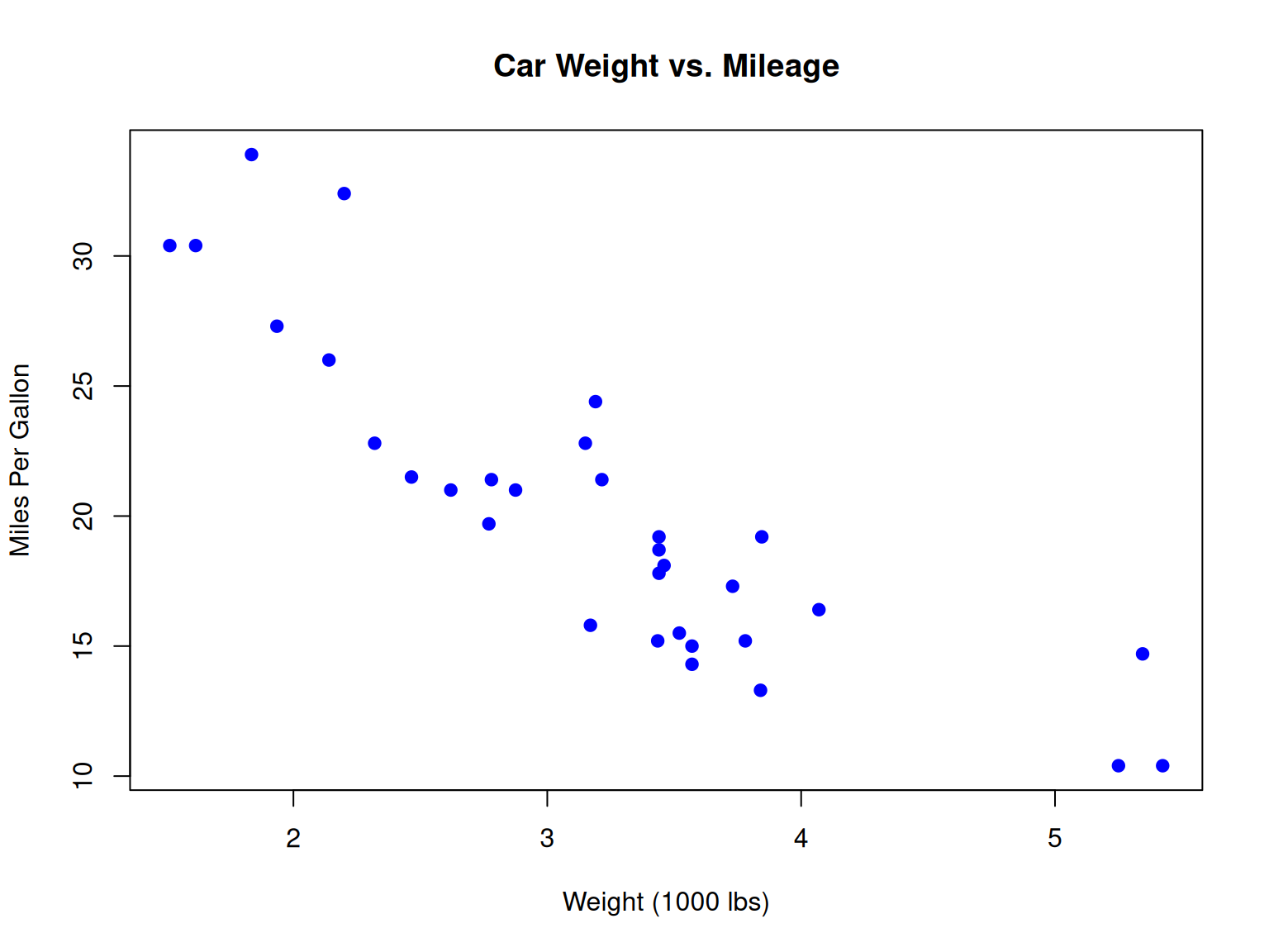
plot(mtcars$wt, mtcars$mpg,
main = "Car Weight vs. Mileage",
xlab = "Weight (1000 lbs)",
ylab = "Miles Per Gallon",
pch = 19, col = "blue")
```
::: {.cell-output-display}
{width=100%}
:::
:::
### Grouped Analysis
::: {.cell}
```{.r .cell-code}
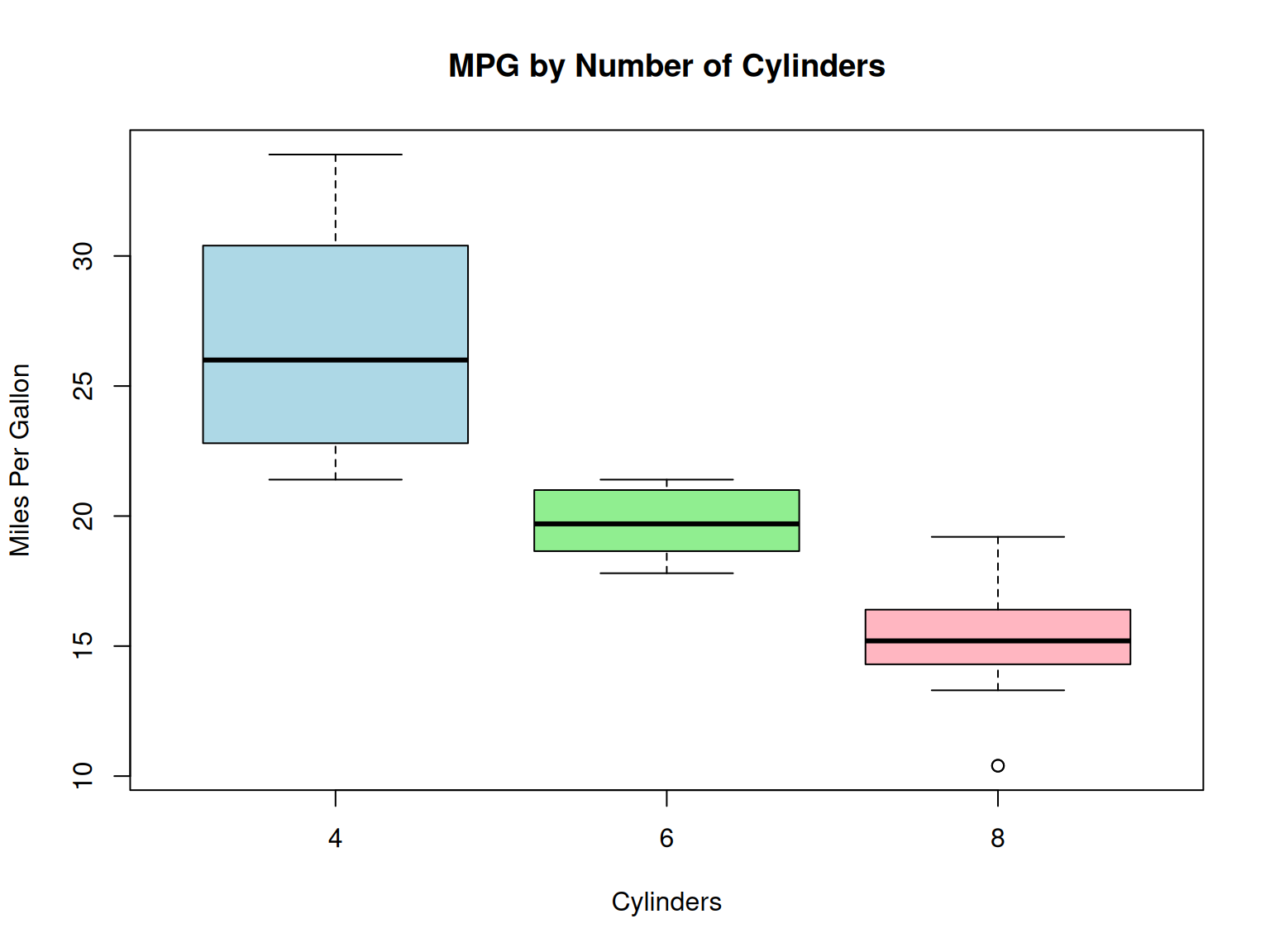
# Add a categorical variable
mtcars$cyl_factor <- as.factor(mtcars$cyl)
# Boxplot by cylinder groups
boxplot(mpg ~ cyl_factor, data = mtcars,
main = "MPG by Number of Cylinders",
xlab = "Cylinders",
ylab = "Miles Per Gallon",
col = c("lightblue", "lightgreen", "lightpink"))
```
::: {.cell-output-display}
{width=100%}
:::
:::
# Statistical Analysis
## Linear Regression
::: {.cell}
```{.r .cell-code}
# Fit a linear model
model <- lm(mpg ~ wt + hp, data = mtcars)
# Display model summary
summary(model)
```
::: {.cell-output .cell-output-stdout}
```
#>
#> Call:
#> lm(formula = mpg ~ wt + hp, data = mtcars)
#>
#> Residuals:
#> Min 1Q Median 3Q Max
#> -3.941 -1.600 -0.182 1.050 5.854
#>
#> Coefficients:
#> Estimate Std. Error t value Pr(>|t|)
#> (Intercept) 37.22727 1.59879 23.285 < 2e-16 ***
#> wt -3.87783 0.63273 -6.129 1.12e-06 ***
#> hp -0.03177 0.00903 -3.519 0.00145 **
#> ---
#> Signif. codes: 0 '***' 0.001 '**' 0.01 '*' 0.05 '.' 0.1 ' ' 1
#>
#> Residual standard error: 2.593 on 29 degrees of freedom
#> Multiple R-squared: 0.8268, Adjusted R-squared: 0.8148
#> F-statistic: 69.21 on 2 and 29 DF, p-value: 9.109e-12
```
:::
:::
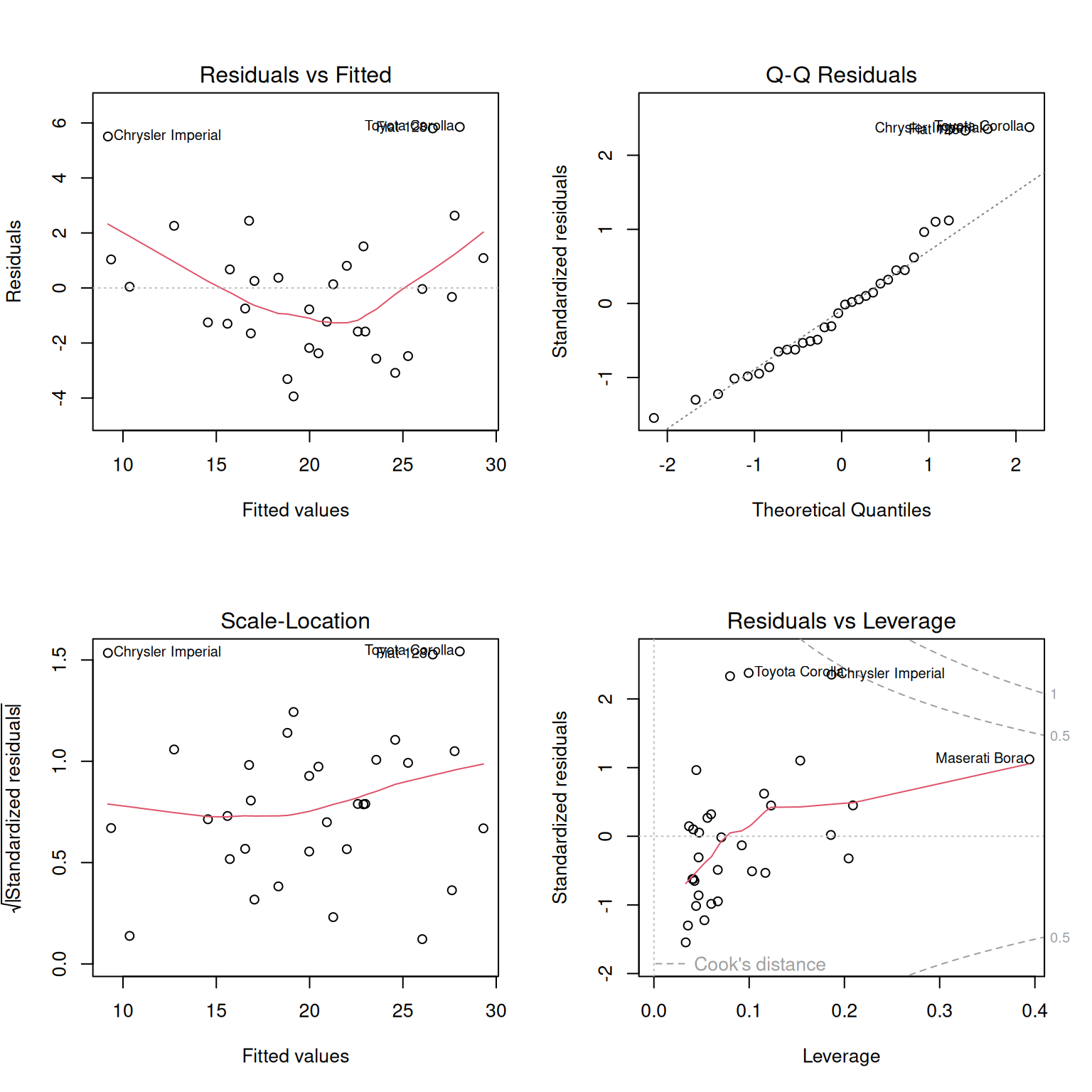
## Diagnostic Plots
::: {.cell}
```{.r .cell-code}
par(mfrow = c(2, 2))
plot(model)
```
::: {.cell-output-display}
{width=100%}
:::
:::
# Conclusion
This document has demonstrated several advanced R Markdown features:
1. A floating table of contents with section numbering
2. Code folding (try clicking the "Code" buttons)
3. The Flatly theme with Tango syntax highlighting
4. Customized chunk options
5. Multi-level headings that appear in the TOCKey features implemented:
-
Table of Contents:
-
toc: trueenables the table of contents -
toc_float: collapsed: false, smooth_scroll: truecreates a floating TOC -
toc_depth: 3includes headings up to level 3 -
number_sections: trueadds numbering to sections
-
-
Code Folding:
-
code_folding: showmakes code chunks expandable/collapsible - Default is to show code, but readers can hide it
-
-
Custom Theme:
-
theme: flatlysets the document theme (other options include “default”, “cerulean”, “journal”, “lumen”, etc.) -
highlight: tangosets the code highlighting style
-
-
Additional Features:
-
df_print: pagedcreates interactive tables for data frames - The setup chunk configures global options for all code chunks
-